Working with Raster Data
GDAL Formats and Drivers
GDAL provides support for a wide-range of raster file formats through the use of drivers which contain specifications and capabilities for handling data. The list of raster drivers currently supported by GDAL can be found here
https://gdal.org/drivers/raster/index.html.
To view a list of available raster formats, run the following command
$ gdal_translate --formats
Exploring Data (gdalinfo)
Use gdalinfo to list information about raster data. This will output data properties including file format, projection, extent, metadata, and raster band information
GeoTIFFs
Let’s explore this 1987 aerial photograph of San Francisco
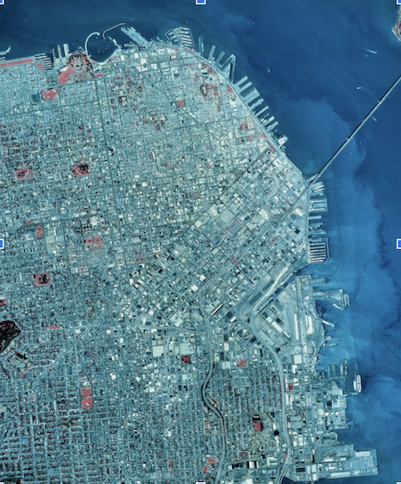
Run the following command
$ gdalinfo SF1987.tif
You should see a large block of output text, beginning with
Driver: GTiff/GeoTIFF
This shows that the file is a GeoTIFF. The next lines of text display the filename, and the image size (in pixels)
Files: SF1987.tif
Size is 6244, 7581
Below that is the projection information. This is the information that places this image correctly over the northeast section of San Francisco, and specifies the location of each pixel.
Coordinate System is:
PROJCRS["NAD83 / UTM zone 10N",
    BASEGEOGCRS["NAD83",
        DATUM["North American Datum 1983",
            ELLIPSOID["GRS 1980",6378137,298.257222101,
                LENGTHUNIT["metre",1]]],
        PRIMEM["Greenwich",0,
            ANGLEUNIT["degree",0.0174532925199433]],
        ID["EPSG",4269]],
    CONVERSION["UTM zone 10N",
        METHOD["Transverse Mercator",
            ID["EPSG",9807]],
        PARAMETER["Latitude of natural origin",0,
            ANGLEUNIT["degree",0.0174532925199433],
            ID["EPSG",8801]],
        PARAMETER["Longitude of natural origin",-123,
            ANGLEUNIT["degree",0.0174532925199433],
            ID["EPSG",8802]],
        PARAMETER["Scale factor at natural origin",0.9996,
            SCALEUNIT["unity",1],
            ID["EPSG",8805]],
        PARAMETER["False easting",500000,
            LENGTHUNIT["metre",1],
            ID["EPSG",8806]],
        PARAMETER["False northing",0,
            LENGTHUNIT["metre",1],
            ID["EPSG",8807]]],
There is also some generic metadata for the file
Metadata:
  AGENCY=WESTERN MAPPING CENTER (WMC) oversight agency*
  AREA_OR_POINT=Area
  DATA_FILE_SIZE=142026024 data set size in bytes*
  EAST_LONGITUDE=-122 22 30.000 signed deg min sec SDDD MM SS.SSS*
  IMAGE_SOURCE=COLOR INFRA-RED FILM b&w, cir, natural color, other*
  METADATA_DATE=1998 4 7 date created or changed, yyyy mm dd*
  NATION=US nation code*
  NE_QUAD_CORNER_XY=555013.021 4185195.796 XY coords. of pri. NE quad corner*
  NORTH_LATITUDE=37 48 45.000 signed deg min sec SDDD MM SS.SSS*
  NW_QUAD_CORNER_XY=549511.672 4185160.843 XY coords. of pri. NW quad corner*
  PRODUCER=WESTERN MAPPING CENTER (WMC)
  PRODUCTION_DATE=1998 1 29 yyyy mm dd*
  PRODUCTION_SYSTEM=DV2.6.3 10/9OV2.4 5/95 production system*
  QUADRANGLE_NAME=SAN FRANCISCO NORTH 3.45 or 7.5-min. name*
  QUADRANT=SE quadrant indicator if cell size = 3.75-minutes*
  RASTER_ORDER=LEFT_RIGHT/TOP_BOTTOM video display order*
  RMSE_XY=3.40 doq horiz. accuracy*
  SECONDARY_HORIZONTAL_DATUM=NAD27 secondary horizontal datum*
  SECONDARY_NE_QUAD_XY=555014.390 4184990.576 XY coords. - sec. NE quad cor.*
  SECONDARY_NW_QUAD_XY=549512.904 4184955.623 XY coords. - sec. NW quad cor.*
  SECONDARY_SE_QUAD_XY=555060.733 4178056.378 XY coords. - sec. SE quad cor.*
  SECONDARY_SW_QUAD_XY=549554.612 4178021.444 XY coords. - sec. SW quad cor.*
  SECONDARY_XY_ORIGIN=549211.000 4185301.000 coord upper left pixel sec datum*
  SE_QUAD_CORNER_XY=555059.365 4178261.445 XY coords. of pri. SE quad corner*
  SOURCE_DEM_DATE=1998 1 29 source dem date yyyy mm dd*
  SOURCE_IMAGE_DATE=1987 6 22 source image date as yyyy mm dd*
  SOURCE_IMAGE_ID=NAPP 511 125 source image id*
  SOUTH_LATITUDE=37 45 0.000 signed deg min sec SDDD MM SS.SSS*
  STANDARD_VERSION=1996 12 version of DOQ standard*
  STATE=CA state fip code*
  SW_QUAD_CORNER_XY=549553.381 4178226.512 XY coords. of pri. SW quad corner*
  WEST_LONGITUDE=-122 26 15.000 signed deg min sec SDDD MM SS.SSS*
The last block of output shows the corner points of the image in two different units (meters and minutes, degrees, seconds), as well as some information about each band (a.k.a. channel). Each channel is byte (8-bit) format, there are three bands (red, green, and blue, respectively).
Corner Coordinates:
Upper Left  (  549115.000, 4185497.000) (122d26'31.14"W, 37d48'55.98"N)
Lower Left  (  549115.000, 4177916.000) (122d26'32.99"W, 37d44'50.01"N)
Upper Right (  555359.000, 4185497.000) (122d22'15.77"W, 37d48'54.70"N)
Lower Right (  555359.000, 4177916.000) (122d22'17.85"W, 37d44'48.73"N)
Center      (  552237.000, 4181706.500) (122d24'24.44"W, 37d46'52.37"N)
Band 1 Block=6244x1 Type=Byte, ColorInterp=Red
Band 2 Block=6244x1 Type=Byte, ColorInterp=Green
Band 3 Block=6244x1 Type=Byte, ColorInterp=Blue
Run gdalinfo on the 1938 Composite image of San Francisco. Notice that each band (RGB) has a NoData Value of 0.
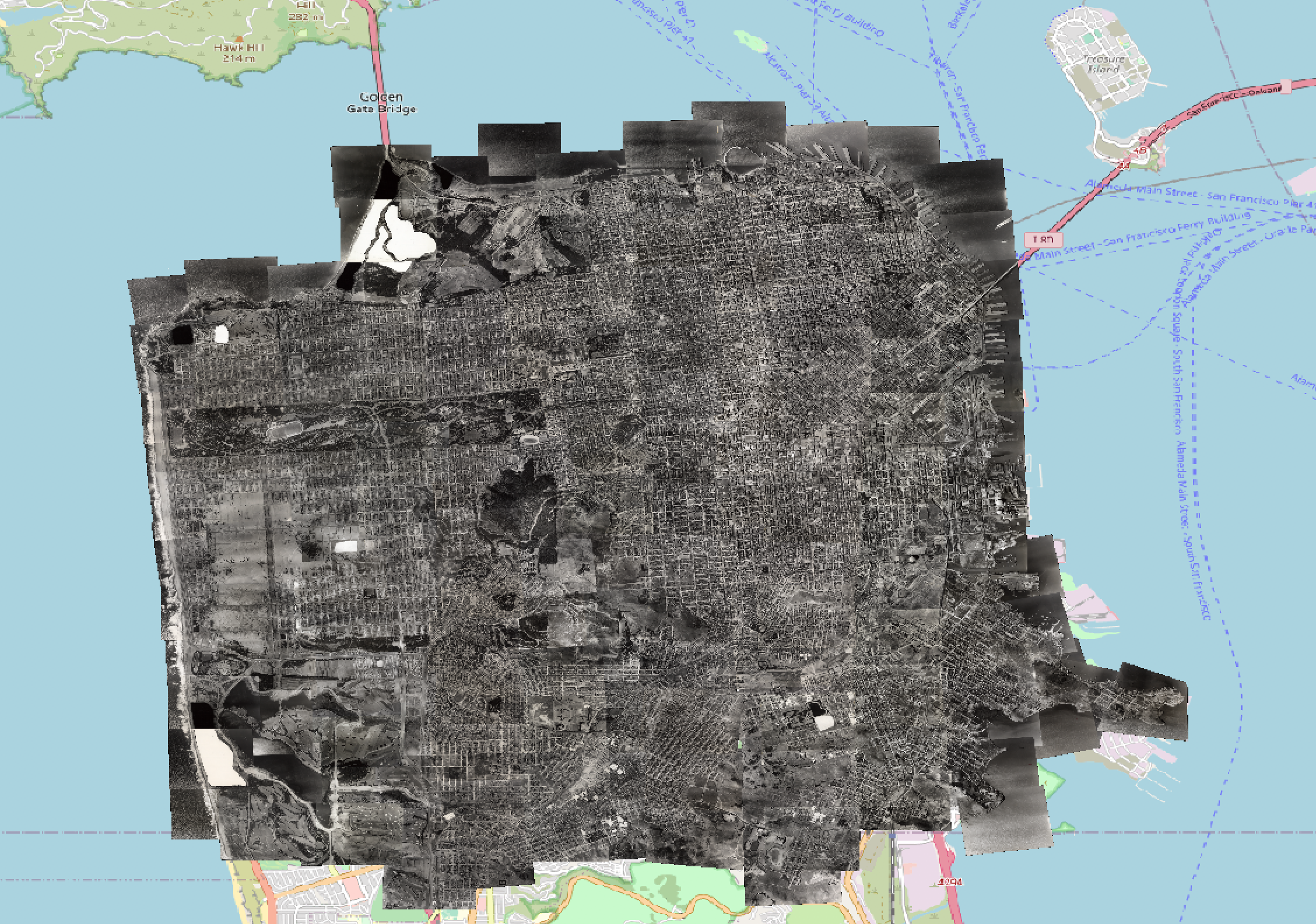
$ gdalinfo SF1938.tif
Band 1 Block=37509x16 Type=Byte, ColorInterp=Red
  Min=1.000 Max=255.000
  Minimum=1.000, Maximum=255.000, Mean=98.291, StdDev=51.897
  NoData Value=0
  Metadata:
    STATISTICS_COVARIANCES=2693.285955948338,2651.095395949078,2569.287814804031
    STATISTICS_MAXIMUM=255
    STATISTICS_MEAN=98.290836665212
    STATISTICS_MINIMUM=1
    STATISTICS_SKIPFACTORX=1
    STATISTICS_SKIPFACTORY=1
    STATISTICS_STDDEV=51.896878094432
Band 2 Block=37509x16 Type=Byte, ColorInterp=Green
  Min=1.000 Max=255.000
  Minimum=1.000, Maximum=255.000, Mean=95.146, StdDev=51.271
  NoData Value=0
  Metadata:
    STATISTICS_COVARIANCES=2651.095395949078,2628.756783663635,2542.154359436107
    STATISTICS_MAXIMUM=255
    STATISTICS_MEAN=95.146410610285
    STATISTICS_MINIMUM=1
    STATISTICS_SKIPFACTORX=1
    STATISTICS_SKIPFACTORY=1
    STATISTICS_STDDEV=51.27140317627
Band 3 Block=37509x16 Type=Byte, ColorInterp=Blue
  Min=1.000 Max=255.000
  Minimum=1.000, Maximum=255.000, Mean=91.934, StdDev=49.754
  NoData Value=0
  Metadata:
    STATISTICS_COVARIANCES=2569.287814804031,2542.154359436107,2475.508464661893
    STATISTICS_MAXIMUM=255
    STATISTICS_MEAN=91.933985832391
    STATISTICS_MINIMUM=1
    STATISTICS_SKIPFACTORX=1
    STATISTICS_SKIPFACTORY=1
    STATISTICS_STDDEV=49.754481855024
Let’s explore the 1915 Map of San Francisco
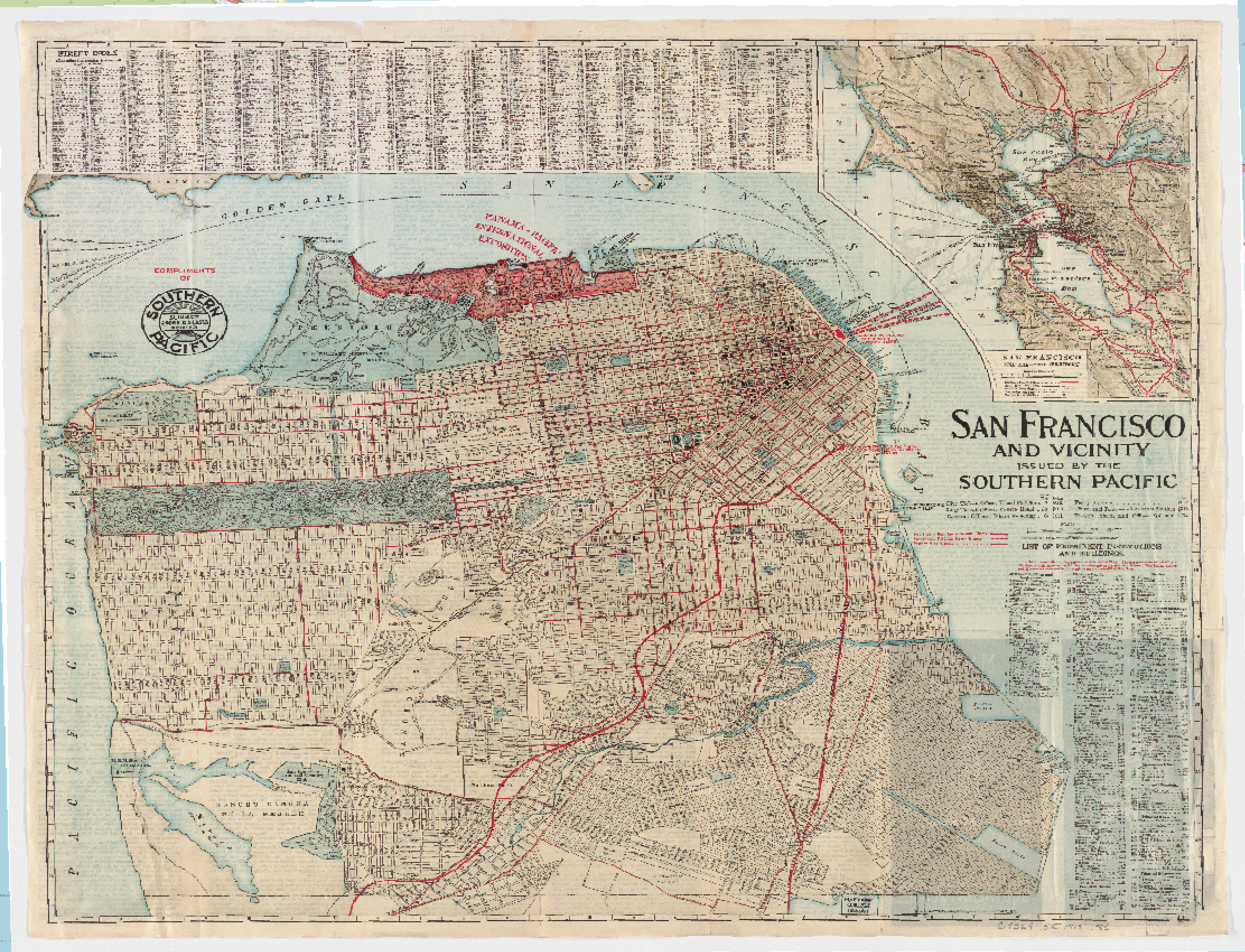
$ gdalinfo SF1915.tif
Notice that there are 4 bands in this image (red, green, blue, alpha), as well as a NoData value of 0
Band 1 Block=4096x8 Type=Byte, ColorInterp=Red
  NoData Value=0
Band 2 Block=4096x8 Type=Byte, ColorInterp=Green
  NoData Value=0
Band 3 Block=4096x8 Type=Byte, ColorInterp=Blue
  NoData Value=0
Band 4 Block=4096x8 Type=Byte, ColorInterp=Alpha
  NoData Value=0
Use the -nomd flag to supress output of metadata
$ gdalinfo -nomd SF1915.tif
Digital Elevation Models
Let’s look at the information for this digital elevation model

$ gdalinfo gt30w140n40_dem/gt30w140n40.dem
Driver: EHdr/ESRI .hdr Labelled
Files: gt30w140n40_dem/gt30w140n40.dem
       gt30w140n40_dem/gt30w140n40.dem.aux.xml
       gt30w140n40_dem/gt30w140n40.hdr
       gt30w140n40_dem/gt30w140n40.stx
       gt30w140n40_dem/gt30w140n40.prj
Size is 4800, 6000
Coordinate System is:
GEOGCRS["WGS 84",
    DATUM["World Geodetic System 1984",
        ELLIPSOID["WGS 84",6378137,298.257223563,
            LENGTHUNIT["metre",1]]],
    PRIMEM["Greenwich",0,
        ANGLEUNIT["degree",0.0174532925199433]],
    CS[ellipsoidal,2],
        AXIS["geodetic latitude (Lat)",north,
            ORDER[1],
            ANGLEUNIT["degree",0.0174532925199433]],
        AXIS["geodetic longitude (Lon)",east,
            ORDER[2],
            ANGLEUNIT["degree",0.0174532925199433]],
    ID["EPSG",4326]]

   ...

Band 1 Block=4800x1 Type=Int16, ColorInterp=Undefined
  Min=-66.000 Max=4280.000
  Minimum=-66.000, Maximum=4280.000, Mean=1329.977, StdDev=744.157
  NoData Value=-9999
Converting Data (gdal_translate)
The gdal_translate utility can convert, compress, and resample raster data
The -of flag is used to specify the output format. If not specified, the format is guessed from the extension.
Converting a GeoTIFF to a PNG:
$ gdal_translate -of png SF1987.tif SF1987_converted.png
The San Francisco 1938 photo (SF1938.tif) is 464 MB. Let’s compress the image using the creation option flags -co with COMPRESS=JPEG, TILED=YES and PHOTOMETRIC=YCBCR to create a compressed, tiled, YCBCR photometric GeoTIFF. YCBCR photometric interpretation will allow for a significant reduction in output size with minimal changes on the color/images. TILED=YES forces creation of tiled files.
$ gdal_translate -co COMPRESS=JPEG -co TILED=YES -co PHOTOMETRIC=YCBCR SF1938.tif SF1938_compressed.tif
The resulting file size is 157.4 MB. Run gdalinfo to see the new information
gdalinfo SF1938_compressed.tif
Understanding Compression of Geospatial Raster Imagery
Warping Data (gdalwarp)
The gdalwarp utility is used for reprojection and image mosaicing. It can reproject to any supported projection, and can also apply ground control points stored with the image if the image is “raw” with control information.
Reprojecting Data
$ gdalwarp -t_srs EPSG:4326 SF1987.tif SF1987_wgs84.tif
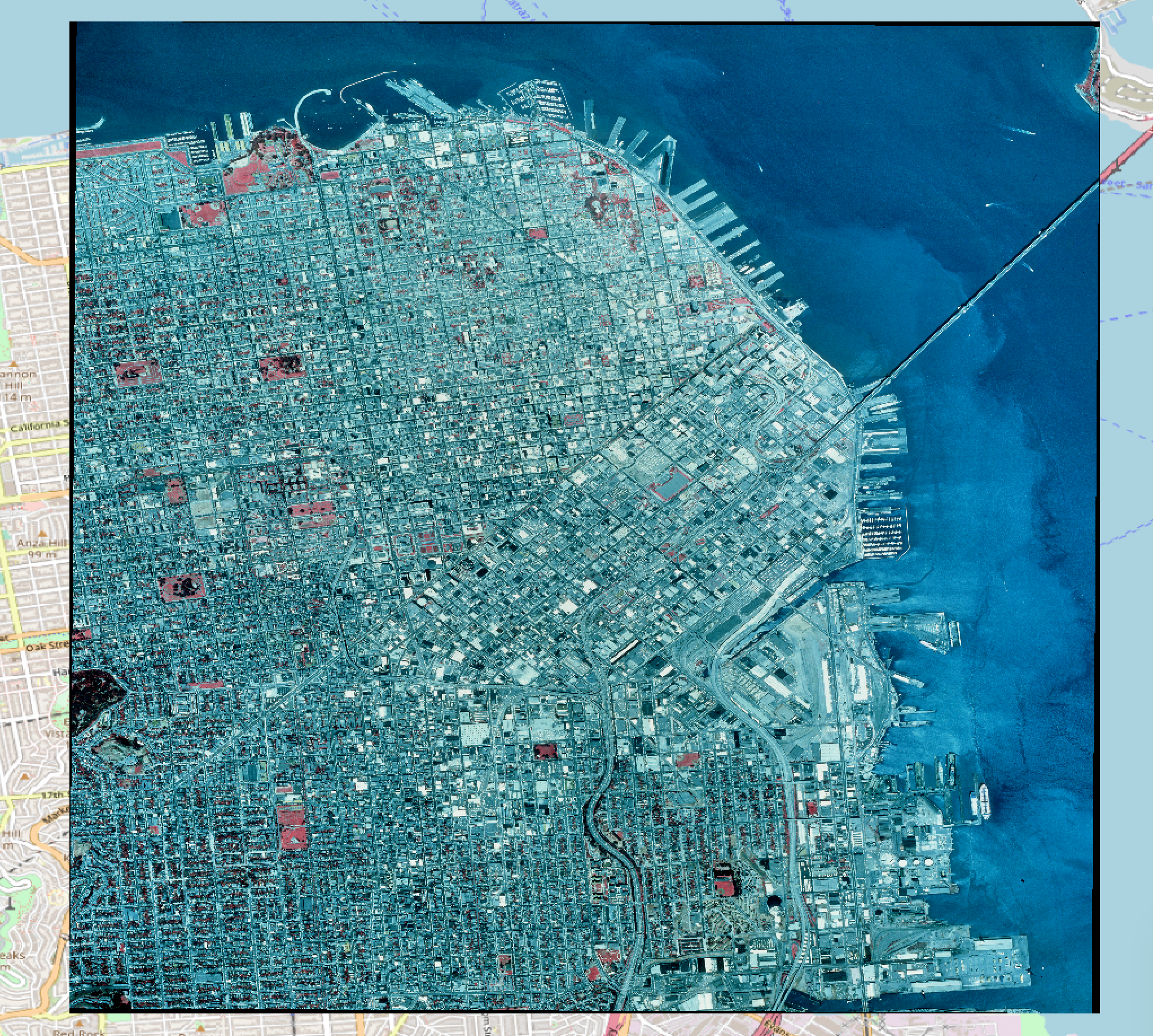
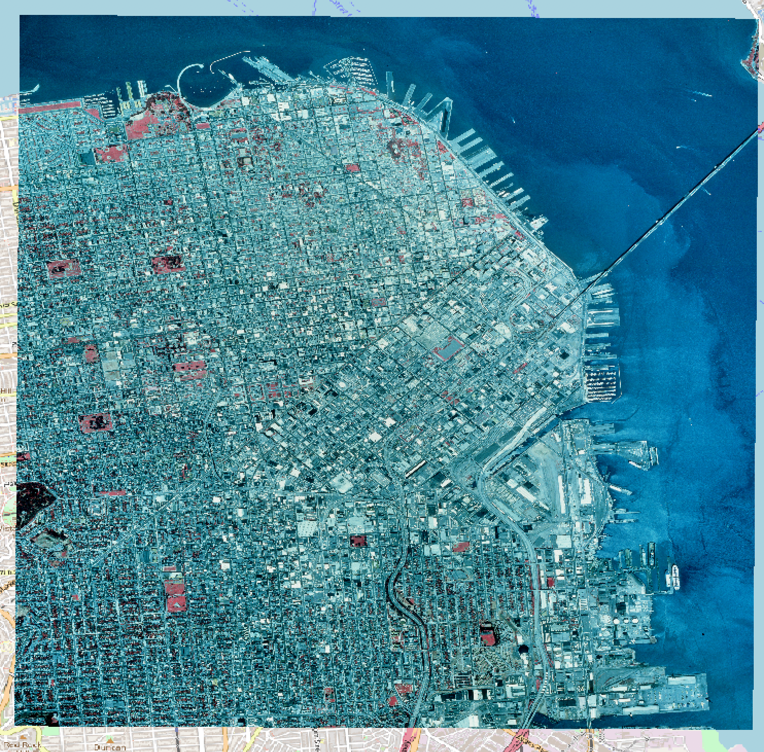
This transformed file contains a black border around the image. This is because the original image did not contain a NoData value, so when the new file is created, black pixels fill in the extent area outside of the image. The simplest way to remedy this is to add a transparency band (alpha channel) to the output file using the -dstalpha flag
$ gdalwarp -t_srs EPSG:4326 -dstalpha -overwrite SF1987.tif SF1987_wgs84.tif
Run gdalinfo on the output to see the information
$ gdalinfo SF1987_wgs84.tif
A 4th band (Alpha) has been added
Band 1 Block=7137x1 Type=Byte, ColorInterp=Red
  Mask Flags: PER_DATASET ALPHA
Band 2 Block=7137x1 Type=Byte, ColorInterp=Green
  Mask Flags: PER_DATASET ALPHA
Band 3 Block=7137x1 Type=Byte, ColorInterp=Blue
  Mask Flags: PER_DATASET ALPHA
Band 4 Block=7137x1 Type=Byte, ColorInterp=Alpha
Batch Processing
Performing the same operation on multiple raster files
Reproject all GeoTIFFs to WGS_84 and add an alpha channel
$ python projectTiffs.py
import os
import fnmatch

INPUT_FOLDER="."
OUTPUT_FOLDER= "wgs84"
if not os.path.exists('wgs84'):
    os.makedirs('wgs84')

def findRasters (path, filter):
    for root, dirs, files in os.walk(path):
        for file in fnmatch.filter(files, filter):
            yield file
        break

for raster in findRasters(INPUT_FOLDER, '*.tif'):
    newFile = raster[:-4]
    inRaster = INPUT_FOLDER + '/' + raster
    outRaster = OUTPUT_FOLDER +'/' + newFile + '_wgs84.tif'
    cmd = 'gdalwarp -t_srs EPSG:4326 -te xmin ymin xmax ymax -dstalpha -overwrite %s %s' % (inRaster, outRaster)
    os.system(cmd)